Deploy machine learning models with GKE and Dataiku

Introduction

In a previous post I described how easy it is to create and deploy machine learning models (exposing them as REST APIs) with Dataiku. In particular, it was an XGboost model predicting home values. Now, suppose my model for predicting home values becomes so successful that I need to serve millions of request per hour, then it would be very handy if my back end scales easily.

In this brief post I outline the few steps you need to take to deploy machine learning models created with Dataiku on a scalable kubernetes cluster on Google Kubernetes Engine (GKE).

Create a Kubernetes cluster

There is a nice GKE quickstart that demonstrate the creation of a kubernetes cluster on Google Cloud Platform (GCP). The cluster can be created by using the GUI on the Google cloud console. Alternatively, if you are making use of the Google cloud SDK, it basically boils down to creating and getting credentials with two commands:

gcloud container clusters create myfirst-cluster
gcloud container clusters get-credentials myfirst-cluster

When creating a cluster, there are many options that you can set. I left all options at their default value. It means that only a small cluster of 3 nodes of machine type n1-standard-1 will be created. We can now see the cluster in the Google cloud console.

Setup the Dataiku API Deployer

Now that you have a kubernetes cluster we can easily deploy predictive models with Dataiku. First, you need to create a predictive model. As described in my previous blog, you can do this with the Dataiku software. Then the Dataiku API Deployer, is the component that will take care of the management and actual deployment of your models onto the kubernetes cluster.

The machine where the Dataiku API Deployer is installed must be able to push docker images to your Google cloud environment and must be able to interact with the kubernetes cluster (through the kubectl command).

Deploy your stuff……

My XGboost model created in Dataiku is now pushed to the Dataiku API Deployer. From the GUI of the API Deployer you are now able to select the XGboost model to deploy it on your kubernetes cluster.

The API Deployer is a management environment to see what models (and model versions) are already deployed, it checks if the models are up and running, it manages your infrastructure (kubernetes clusters or normal machines).

When you select a model that you wish to deploy, you can click deploy and select a cluster. It will take a minute or so to package that model into a Docker image and push it to GKE. You will see a progress window.

When the process is finished you will see the new service on your Kubernetes Engine on GCP.

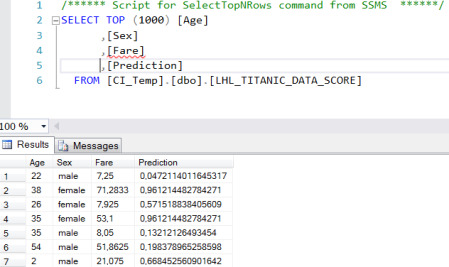
The model is up and running, waiting to be called. You could call it via curl for example:

curl -X POST \
  http://35.204.180.188:12000/public/api/v1/xgboost/houseeprice/predict \
  --data '{ "features" : {
    "HouseType": "Tussenwoning",
      "kamers": 6,
      "Oppervlakte": 134,
      "VON": 0,
      "PC": "16"
  }}'

Conclusion

That’s all it was! You now have a scalable model serving engine. Ready to be easily resized when the millions of requests start to come in….. Besides predictive models you can also deploy/expose any R or Python function via the Dataiku API Deployer. Don’t forget to shut down the cluster to avoid incurring charges to your Google Cloud Platform account.

gcloud container clusters delete myfirst-cluster

Cheers, Longhow.

Cucumber time, food on a 2D plate / plane

Introduction

It is 35 degree Celsius out side, we are in the middle of the ‘slow news season’, in many countries also called cucumber time.  A period typified by the appearance of less informative and frivolous news in the media.

Did you know that 100 g of cucumber contain 0.28 mg of iron and 1.67 g of sugar? You can find all the nutrient values of a cucumber on the USDA food databases.

Food Data

There is more data, for many thousands of products you can retrieve nutrient values through an API (need to register for a free KEY). So besides the cucumber I extracted data for different type of food for example

• Beef products
• Dairy & Egg products
• Vegetables
• Fruits
• etc.

And as a comparison, I retrieved the nutrient values for some fast food products from McDonald’s and Pizza Hut. Just to see if pizza can be classified  as vegetable from a data point of view 🙂 So the data looks like:

I have sampled 1500 products and per product we have 34 nutrient values.

Results

The 34 dimensional data is now compressed / projected onto a two dimensional plane using UMAP (Uniform Manifold Approximation and Projection). There is a Python and R package to this.

An interactive map can be found here, and the R code to retrieve and plot the data here. Cheers, Longhow.

 

t-sne dimension reduction on Spotify mp3 samples

Introduction

Not long ago I was reading on t-Distributed Stochastic Neighbor Embedding (t-sne), a very interesting dimension reduction technique, and on Mel frequency cepstrum a sound processing technique. Details of both techniques can be found here and here. Can we combine the two in a data analysis exercise? Yes, and with not too much R code you can already quickly create some visuals to get ‘musical’ insights.

Spotify Data

Where can you get some sample audio files? Spotify! There is a Spotify API which allows you to get information on playlists, artists, tracks, etc. Moreover, for many songs (not all though) Spotify provides downloadable preview mp3’s of 30 seconds. The link to the preview mp3 can be retrieved from the API. I am going to use some of these mp3’s for analysis.

In the web interface of Spotify you can look for interesting playlists. In the search field type in for example ‘Bach‘ (my favorite classical composer). In the search results go to the playlists tab, you’ll find many ‘Bach’ playlists from different users, including the ‘user’ Spotify itself. Now, given the user_id (spotify) and the specific playlist_id (37i9dQZF1DWZnzwzLBft6A for the Bach playlist from Spotify) we can extract all the songs using the API:

 GET https://api.spotify.com/v1/users/{user_id}/playlists/{playlist_id}

You will get the 50 Bach songs from the playlist, most of them have a preview mp3. Let’s also get the songs from a Heavy Metal play list, and a Michael Jackson play list. In total I have 146 songs with preview mp3’s in three ‘categories’:

• Bach,
• Heavy Metal,
• Michael Jackson.

Transforming audio mp3’s to features

The mp3 files need to be transformed to data that I can use for machine learning, I am going to use the Python librosa package to do this. It is easy to call it from R using the reticulate package.

library(reticulate)
librosa = import("librosa")

#### python environment with librosa module installed
use_python(python = "/usr/bin/python3")

The downloaded preview mp3’s have a sample rate of 22.050. So a 30 second audio file has in total 661.500 raw audio data points.

onemp3 = librosa$load("mp3songs/bach1.mp3")

length(onemp3[[1]])
length(onemp3[[1]])/onemp3[[2]]  # ~30 seconds sound

## 5 seconds plot
pp = 5*onemp3[[2]]
plot(onemp3[[1]][1:pp], type="l")

A line plot of the raw audio values will look like.

For sound processing, features extraction on the raw audio signal is often applied first. A commonly used feature extraction method is Mel-Frequency Cepstral Coefficients (MFCC). We can calculate the MFCC for a song with librosa.

ff = librosa$feature
mel = librosa$logamplitude(
  ff$melspectrogram(
    onemp3[[1]], 
    sr = onemp3[[2]],
    n_mels=96
  ),
  ref_power=1.0
)
image(mel)

Each mp3 is now a matrix of MFC Coefficients as shown in the figure above. We have less data points than the original 661.500 data points but still quit a lot. In our example the MFCC are a 96 by 1292 matrix, so 124.032 values. We apply a the t-sne dimension reduction on the MFCC values.

Calculating t-sne

A simple and easy approach, each matrix is just flattened. So a song becomes a vector of length 124.032. The data set on which we apply t-sne consist of 146 records with 124.032 columns, which we will reduce to 3 columns with the Rtsne package:

tsne_out = Rtsne(AllSongsMFCCMatrix, dims=3) 

The output object contains the 3 columns, I have joined it back with the data of the artists and song names so that I can create an interactive 3D scatter plot with R plotly. Below is a screen shot, the interactive one can be found here.

Conclusion

It is obvious that Bach music, heavy metal and Michael Jackson are different, you don’t need machine learning to hear that. So as expected, it turns out that a straight forward dimension reduction on these songs with MFCC and t-sne clearly shows the differences in a 3D space. Some Michael Jackson songs are very close to heavy metal 🙂 The complete R code can be found here.

Cheers, Longhow

The ‘I-Love-IKEA’ – web app, built at the IKEA Hackaton with R and Shiny

Introduction

On the 8th, 9th and 10th of December I participated at the IKEA hackaton. In one word it was just FANTASTIC! Well organized, good food, and participants from literally all over the world, even the heavy snow fall on Sunday did not stop us from getting there!

 

I formed a team with Jos van Dongen and his son Thomas van Dongen and we created the “I-Love-IKEA” app to help customers find IKEA products. And of course using R.

The “I-Love-IKEA” Shiny R app

The idea is simple. Suppose you are in the unfortunate situation that you are not in an IKEA store, and you see a chair, or nice piece of furniture, or something completely else…. Now does IKEA have something similar? Just take a picture, upload it using the I-Love-IKEA R Shiny app and get the best matching IKEA products back.

Implementation in R

How was this app created? The following steps outline steps that we took during the creation of the web app for the hackaton.

First, we have scraped 9000 IKEA product images using Rvest, then each image is ‘scored’ using a pre-trained VGG16 network, where the top layers are removed.

 

That means that for each IKEA image we have a 7*7*512 tensor, we flattened this tensor to a 25088 dimensional vector. Putting all these vectors in a matrix we have a 9000 by 25088 matrix.

If you have a new image, we use the same pre-trained VGG16 network to generate a 25088 dimensional vector for the new image. Now we can calculate all the 9000 distances (for example cosine similarity) between this new image and the 9000 IKEA images. We select, say, the top 7 matches.

A few examples

A Shiny web app

To make this useful for an average consumer, we have put it all in an R Shiny app using the library ‘minUI‘ so that the web site is mobile friendly. A few screen shots:

 

The web app starts with an ‘IKEA-style’ instruction, then it allows you to take a picture with your phone, or use one that you already have on your phone. It uploads the image and searches for the best matching IKEA products.

The R code is available from my GitHub, and a live running Shiny app can be found here.

Conclusions

Obviously, there are still many adjustments you can make to the app to improve the matching. For example pre process the images before they are sent through the VGG network. But there was no more time.

Unfortunately, we did not win a price during the hackaton, the jury did however find our idea very interesting. More importantly, we had a lot of fun. In Dutch “Het waren 3 fantastische dagen!”.

Cheers, Longhow.

The one function call you need to know as a data scientist: h2o.automl

Introduction

Two things that recently came to my attention were AutoML (Automatic Machine Learning) by h2o.ai and the fashion MNIST by Zalando Research. So as a test, I ran AutoML on the fashion mnist data set.

H2o AutoML

As you all know a large part of the work in predictive modeling is in preparing the data. But once you have done that, ideally you don’t want to spend too much work in trying many different machine learning models.  That’s were AutoML from h2o.ai comes in. With one function call you automate the process of training a large, diverse, selection of candidate models.

AutoML trains and cross-validates a Random Forest, an Extremely-Randomized Forest, GLM’s, Gradient Boosting Machines (GBMs) and Neural Nets. And then as “bonus” it trains a Stacked Ensemble using all of the models. The function to use in the h2o R interface is: h2o.automl. (There is also a python interface)

FashionMNIST_Benchmark = h2o.automl(
  x = 1:784,
  y = 785,
  training_frame = fashionmnist_train,
  validation_frame = fashionmninst_test
)

So the first 784 columns in the data set are used as inputs and column 785 is the column with labels. There are more input arguments that you can use. For example, maximum running time or maximum number of models to use, a stopping metric.

It can take some time to run all these models, so I have spun up a so-called high CPU droplet on Digital Ocean: 32 dedicated cores ($0.92 /h).

h2o utilizing all 32 cores to create models

The output in R is an object containing the models and a ‘leaderboard‘ ranking the different models. I have the following accuracies on the fashion mnist test set.

1. Gradient Boosting (0.90)
2. Deep learning (0.89)
3. Random forests (0.89)
4. Extremely randomized forests (0.88)
5. GLM (0.86)

There is no ensemble model, because it’s not supported yet for multi label classifiers. The deeplearning in h2o are fully connected hidden layers, for this specific Zalando images data set, you’re better of pursuing more fancy convolutional neural networks. As a comparison I just ran a simple 2 layer CNN with keras, resulting in an test accuracy of 0.92. It outperforms all the models here!

Conclusion

If you have prepared your modeling data set, the first thing you can always do now is to run h2o.automl.

Cheers, Longhow.

A “poor man’s video analyzer”…

Introduction

Not so long ago there was a nice dataiku meetup with Pierre Gutierrez talking about transfer learning. RStudio recently released the keras package, an R interface to work with keras for deep learning and transfer learning. Both events inspired me to do some experiments at my work here at RTL and explore the usability of it for us at RTL. I like to share the slides of the presentation that I gave internally at RTL, you can find them on slide-share.

As a side effect, another experiment that I like to share is the “poor man’s video analyzer“. There are several vendors now that offer API’s to analyze videos. See for example the one that Microsoft offers. With just a few lines of R code I came up with a shiny app that is a very cheap imitation 🙂

Set up of the R Shiny app

To run the shiny app a few things are needed. Make sure that ffmpeg is installed, it is used to extract images from a video. Tensorflow and keras need to be installed as well. The extracted images from the video are parsed through a pre-trained VGG16 network so that each image is tagged.

After this tagging a data table will appear with the images and their tags. That’s it! I am sure there are better visualizations than a data table to show a lot of images. If you have a better idea just adjust my shiny app on GitHub…. 🙂

Using the app, some screen shots

There is a simple interface, specify the number of frames per second that you want to analyse. And then upload a video, many formats are supported (by ffmpeg), like *.mp4, *.mpeg, *.mov

Click on video images to start the analysis process. This can take a few minutes, when it is finished you will see a data table with extracted images and their tags from VGG-16.

Click on ‘info on extracted classes’ to see an overview of the class. You will see a bar chart of tags that where found and the output of ffmpeg. It shows some info on the video.

If you have code to improve the data table output in a more fancy visualization, just go to my GitHub.

For those who want to play around, look at a live video analyzer shiny app here.

And Shiny App version using miniUI will be a better fit for small mobile screens.

Cheers, Longhow

Did you say SQL Server? Yes I did….

Introduction

My last blog post in 2016 on SQL Server 2016….. Some years ago, I have heard predictions from ‘experts‘ that within a few years Hadoop / Spark systems would take over traditional RDBMS’s like SQL Server. I don’t think that has happened (yet). Moreover, what some people don’t realize is that at least half of the world still depends on good old SQL Server. If tomorrow all the Transact stored procedures would somehow magically fail to run anymore, I think our society as we know it would collapse…..

OK, I might be exaggerating a little bit. The point is, there are still a lot of companies and use cases out there that are running SQL Server without the need for something else. And now with the integrated R services in SQL Server 2016 that might not be necessary at all 🙂

Deploying Predictive models created in R

From a business standpoint, creating a good predictive model and spending time on this, is only useful if you can deploy such a model in a system where the business can make use of the predictions in their ‘day-to-day operations’. Otherwise creating a predictive model is just an academic exercise / experiment….

Many predictive models are created in R on a ‘stand-alone’ laptop /server. There are different ways to deploy such models. Among others:

• Re-build the scoring logic ‘by hand’ in the operational system. I did this in the past, it can be a little bit cumbersome and it’s not what you really want to do. If you do not have much data prep steps and your model is a logistic regression or a single tree, this is doable 🙂
• Make use of PMML scoring. The idea is to create a model (in R) transform that to pmml and import the pmml in the operational system where you need the predictions. Unfortunately, not all models are supported and not all systems support importing (the latest version of) PMML
• Create API’s (automatically) with technology like for example Azure ML, DeployR, sense.io or openCPU, so that the application that needs the prediction can call the API.

SQL Server 2016 R services

If your company is running SQL Server (2016) there is an other nice alternative to deploy R models by using the SQL Server R services. At my work at RTL Nederland [Oh btw we are looking for data engineers and data scientists :-)] we are using this technology to deploy the predictive churn and response models created in R. The process is not difficult; the few steps that are needed are demonstrated below.

Create any model in R

I am using an extreme gradient boosting algorithm to fit a classification model on the titanic data set. Instead of calling xgboost directly I am using the mlr package to train the model. Mlr provides a unified interface to machine learning in R, it takes care of some of the frequently used steps in creating a predictive model regardless of the underlying machine learning algorithm. So your code can become very compact and uniform.

Push the (xgboost) predictive model to SQL Server

Once you are satisfied with the predictive model (on your R laptop), you need to bring that model over to SQL Server so that you can use it there. This consists of the following steps:

SQL Code in SQL Server, write a stored procedure in SQL server that can accept a predictive R model, some meta data and saves that into a table in SQL Server.

This stored procedure can then be called from your R session.

Bring the model from R to SQL, to make it a little bit easier you can write a small helper function.

So what is the result? In SQL Server I now have a table (dbo.R_Models) with predictive models. My xgboost model to predict the survival on the Titanic is now added as an extra row. Such a table becomes like a sort of model store in SQL server.

Apply the predictive model in SQL Server.

Now that we have a model we can use it to calculate model scores on data in SQL Server. With the new R services in SQL Server 2016 there is a function called sp_exec_external_script. In this function you can call R to calculate model scores.

The scores (and the inputs) are stored added in a table.

The code is very generic, instead of xgboost models it works for any model. The scoring can (and should be) be done inside a stored procedure so that scoring can be done at regular intervals or triggered by certain events.

Conclusion

Deploying predictive models (that are created in R) in SQL Server has become easy with the new SQL R services. It does not require new technology or specialized data engineers. If your company is already making use of SQL Server then integrated R services are definitely something to look at if you want to deploy predictive models!

Some more examples with code can be found on the Microsoft GitHub pages.

Cheers, Longhow

Don’t give up on single trees yet…. An interactive tree with Microsoft R

Introduction

A few days ago Microsoft announced their new Microsoft R Server 9.0 version. Among a lot of new things, it includes some new and improved machine learning algorithms in their MicrosoftML package.

• Fast linear learner, with support for L1 and L2 regularization. Fast boosted decision tree. Fast random forest. Logistic regression, with support for L1 and L2 regularization.
• GPU-accelerated Deep Neural Networks (DNNs) with convolutions. Binary classification using a One-Class Support Vector Machine.

And the nice thing is, the MicrosoftML package is now also available in the Microsoft R client version, which you can download and use for free.

Don’t give up on single trees yet….

Despite all the more modern machine learning algorithms, a good old single decision tree can still be useful. Moreover, in a business analytics context they can still keep up in predictive power. In the last few months I have created different predictive response and churn models. I usually just try different learners, logistic regression models, single trees, boosted trees, several neural nets, random forests. In my experience a single decision tree is usually ‘not bad’, often only slightly less predictive power than the more fancy algorithms.

An important thing in analytics is that you can ‘sell‘ your predictive model to the business. A single decision tree is a good way to to do just that, and with an interactive decision tree (created by Microsoft R) this becomes even more easy.

Here is an example: a decision tree to predict the survival of Titanic passengers.

The interactive version of the decision tree can be found on my GitHub.

Cheers, Longhow

Danger, Caution H2O steam is very hot!!

H2O has recently released its steam AI engine, a fully open source engine that supports the management and deployment of machine learning models. Both H2O on R and H2O steam are easy to set up and use. And both complement each other perfectly.

A very simple example

Use H2O on R to create some predictive models. Well, due to lack of inspiration I just used the iris set to create some binary classifiers.

Once these models are trained, they are available for use in the H2O steam engine. A nice web interface allows you to set up a project in H2O steam to manage and display summary information of the models.

In H2O steam you can select a model that you want to deploy. It becomes a service with a REST API, a page is created to test the service.

And that is it! Your predictive model is up and running and waiting to be called from any application that can make REST API calls.

There is a lot more to explore in H2O steam, but be careful H2O steam is very hot!

A little H2O deeplearning experiment on the MNIST data set

Introduction

H2O is a fast and scalable opensource machine learning platform. Several algorithms are available, for example neural networks, random forests, linear models and gradient boosting. See the complete list here. Recently the H2O world conference was held, unfortunately I was not there. Luckily there is a lot of material available, videos and slides, it triggered me to try the software.

The software is easy to set up on my laptop. Download the software from the H2O download site, it is a zip file that needs to be unzipped. It contains (among other files) a jar file that needs to be run from the command line:

java -jar h20.jar

After H2O has started, you can browse to localhost:54321 (the default port number can be changed, specify: -port 65432) and within the browser you can use H2O via the flow interface. In this blog post I will not use the flow interface but I will use the R interface.

H2O flow web interface

The H2O R interface

To install the H2O R interface you can follow the instructions provided here. Its a script that checks if there is already a H2O R package installed, if needed it installs packages that the H2O package depends on, and it installs the H2O R package. Start the interface to H2O from R. If H2O was already started from the command line you can connect to the same H2O instance by specifying the same port and use startH2O = FALSE.

library(h2o)

localH2O =  h2o.init(nthreads = -1, port = 54321, startH2O = FALSE)

MNIST handwritten digits

The data I have used for my little experiment is the famous handwritten digits data from MNIST. The data in CSV format can be downloaded from Kaggle. The train data set has 42.000 rows and 785 columns, each row represents a digit, a digit is made up of 28 by 28 pixels, in total 784 columns, plus one additional label column. The first column in the CSV file is called ‘label’, the rest of the columns are called called pixel0, pixel1,….,pixel783. The following code imports the data and plots the first 100 digits, together with the label.

MNIST_DIGITStrain = read.csv( 'D:/R_Projects/MNIST/MNIST_DIGITStrain.csv' )
par( mfrow = c(10,10), mai = c(0,0,0,0))
for(i in 1:100){
  y = as.matrix(MNIST_DIGITStrain[i, 2:785])
  dim(y) = c(28, 28)
  image( y[,nrow(y):1], axes = FALSE, col = gray(255:0 / 255))
  text( 0.2, 0, MNIST_DIGITStrain[i,1], cex = 3, col = 2, pos = c(3,4))
}

The first 100 MNIST handwritten digits and the corresponding label

The data is imported into R, its a local R data frame. To apply machine learning techniques on the MNIST digits, the data needs to be available on the H2O platform. From R you can either import a CSV file directly into the H2O platform or you can import an existing R object into the H2O platform.

mfile = 'D:\\R_Projects\\MNIST\\MNIST_DIGITStrain.csv'
MDIG = h2o.importFile(path = mfile,sep=',')

# Show the data objects on the H2O platform
h2o.ls()

key
1 MNIST_DIGITStrain.hex_3

Deep learning autoencoder

Now that the data is in H2O we can apply machine learning techniques on the data. One type of analysis that interested me the most is the ability to train autoencoders. The idea is to use the input data to predict the input data by means of a ‘bottle-neck’ network.

The middle layer can be regarded as a compressed representation of the input. In H2O R, a deep learning autoencoder can be trained as follows.

NN_model = h2o.deeplearning(
  x = 2:785,
  training_frame = MDIG,
  hidden = c(400, 200, 2, 200, 400 ),
  epochs = 600,
  activation = 'Tanh',
  autoencoder = TRUE
)

So there is one input layer with 784 neurons, a second layer with 400 neurons, a third layer with 200, the middle layer with 2 neurons, etc. The middle layer is a 2-dimensional representation of a 784 dimensional digit. The 42.000 2-dimensional representations of the digits are just points that we can plot. To extract the data from the middle layer we need to use the function h20.deepfeatures.

train_supervised_features2 = h2o.deepfeatures(NN_model, MDIG, layer=3)

plotdata2 = as.data.frame(train_supervised_features2)
plotdata2$label = as.character(as.vector(MDIG[,1]))

qplot(DF.L3.C1, DF.L3.C2, data = plotdata2, color = label, main = 'Neural network: 400 - 200 - 2 - 200 - 400')

In training the autoencoder network I have not used the label, this is not a supervised training exercise. However, I have used the label in the plot above. We can see the ‘1’ digits clearly on the left-hand side, while the ‘7’ digits are more on the right-hand side, and the pink ‘8’ digits are more in the center. It’s far from a perfect, I need to explore more options in the deep learning functionality to achieve a better separation in 2 dimensions.

Comparison with a 2 dimensional SVD data reduction

Autoencoders use nonlinear transformations to compress high dimensional data to a lower dimensional space. Singular Value decomposition on the other hand can be used to compress data to a lower dimensional space by using only linear transformations. See my earlier blog post on SVD. The following picture shows the MNIST digits projected to 2 dimensions using SVD.

There is a good separation between the 1’s and the 0’s, but the rest of the digits are much less separated than the autoencoder. There is of course a time benefit for the SVD. It takes around 6.5 seconds to calculate a SVD on the MNIST data while it took around 350 seconds for the autoencoder.

Conclusion

With this little autoencoder example, I have just scratched the surface of what is possible in H2O. There is much more to discover, many supervised learning algorithms, and also within the deep learning functionality of H2O there are a lot of settings which I have not explored further.